1. How to evaluate the performance of a machine learning model?

Let us consider a task to classify whether a player is a purchaser or not. If the player completes an in-app purchase on store purchase status is positive (+ve ). When don't complete the in-app purchase, the status is negative (-ve), then the person is not the purchaser.

Now consider the above classification ( purchaser or not purchaser) carried out by a machine learning algorithm. The output of the machine learning algorithm can be mapped to one of the following categories.

1.1. A person who is actually a purchaser (positive) and classified as a purchaser (positive). This is called TRUE POSITIVE ( TP).

Figure 1: True Positive.

1.2. A person who is actually not purchaser (negative) and classified as not purchaser (negative). This is called TRUE NEGATIVE ( TN).

Figure 2: True Negative.

1.3. A person who is actually not purchaser (negative) and classified as purchaser (positive). This is called FALSE POSITIVE ( FP).

1.4. A person who is actually a purchaser (positive) and classified as not a purchaser (negative). This is called FALSE NEGATIVE ( FN).

What we desire is TRUE POSITIVE and TRUE NEGATIVE but due to the misclassifications, we may also end up in FALSE POSITIVE and FALSE NEGATIVE. So there is confusion in classifying whether a player is a purchaser or not. This is because no machine learning algorithm is perfect. Soon we will describe this confusion in classifying the data in a matrix called confusion matrix.

Now, we select 100 players which include the purchaser, non-purchaser. Let us assume out of this 100 players 40 are purchasers and the remaining 60 players include non- purchaser. We now use a machine-learning algorithm to predict the outcome. The predicted outcome ( purchaser+ve or -ve) using a machine learning algorithm is termed as the predicted label and the true outcome is termed as the true label .

Now we will introduce the confusion matrix which is required to compute the accuracy of the machine learning algorithm in classifying the data into its corresponding labels.

The following diagram illustrates the confusion matrix for a binary classification problem.

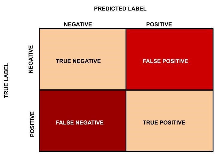
Figure 5: Confusion Matrix.

We will now go back to the earlier example of classifying 100 players (which includes 40 purchasers and the remaining 60 are non-purchasers) as the purchaser or non-purchaser. Out of 40 purchaser players 30 purchaser players are classified correctly and the remaining 10 are classified as non- purchaser by the machine learning algorithm. On the other hand, out of 60 players in the not purchasers category, 55 are classified as non-purchaser and the remaining 5 are classified as the purchaser.

In this case, TN = 55, FP = 5, FN = 10, TP = 30. The confusion matrix is as follows.

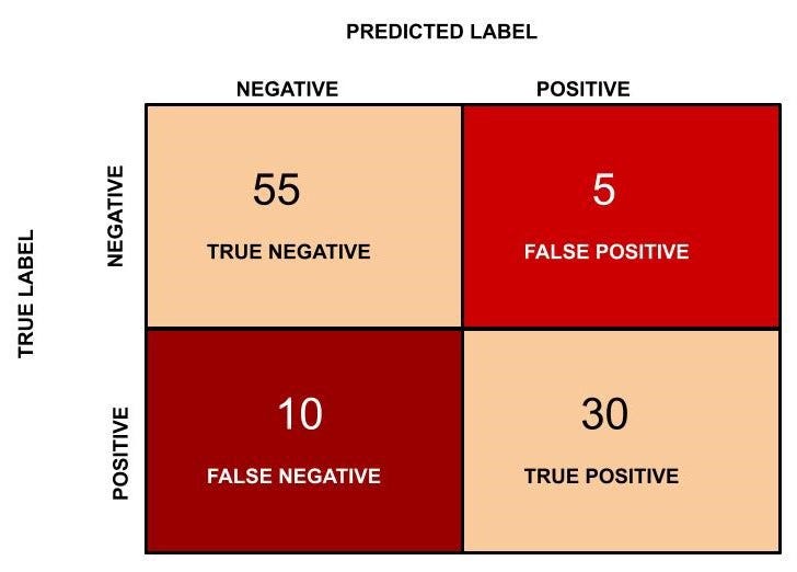
Figure 6: Confusion matrix for the purchaser vs non- purchaser classification.

2. What is the Accuracy of the AppNava Machine Learning model for classification?

Accuracy represents the number of correctly classified data instances over the total number of data instances.

In this example, Accuracy = (55 + 30)/(55 + 5 + 30 + 10 ) = 0.85 and in percentage the accuracy will be 85%.

3. Is Accuracy enough alone?

Accuracy may not be a good measure if the dataset is not balanced (both negative and positive classes have different numbers of data instances). We will explain this with an example.

Consider the following scenario: There are 90 players who are non-purchaser (negative) and 10 players who are purchaser (positive). Now let’s say our machine learning model perfectly classified the 90 players as non-purchaser, but it also classified the purchaser people as non-purchaser. What will happen in this scenario? Let us see the confusion matrix and find out the accuracy?

In this example, TN = 90, FP = 0, FN = 10 and TP = 0. The confusion matrix is as follows.

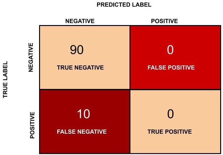
Figure 7: Confusion matrix for purchaser vs non- purchaser player classification.

Accuracy in this case will be (90 + 0)/(100) = 0.9 and in percentage the accuracy is 90 %.

4. Is there anything wrong?

The accuracy, in this case, is 90 % but this model is very poor because all the 10 players who are purchaser are classified as non- purchaser. By this example what we are trying to say is that accuracy is not a good metric when the data set is unbalanced. Using accuracy in such scenarios can result in a misleading interpretation of results.

Now we will find the precision (positive predictive value) in classifying the data instances. Precision is defined as follows:

5. What does Precision mean?

Precision should ideally be 1 for a good classifier. Precision becomes 1 only when the numerator and denominator are equal i.e TP = TP +FP , this also means FP is zero. As FP increases the value of the denominator becomes greater than the numerator and the precision value decreases.

So in the purchaser example, precision = 30/(30+ 5) = 0.857

Now we will introduce another important metric called recall . The recall is also known as sensitivity or true positive rate and is defined as follows:

Recall should ideally be 1 for a good classifier. Recall becomes 1 only when the numerator and denominator are equal i.e TP = TP +FN , this also means FN is zero. As FN increases the value of the denominator becomes greater than the numerator and the recall value decreases (which we don’t want).

So in the purchaser example let us see what will be the recall.

Recall = 30/(30+ 10) = 0.75

So ideally in a good classifier, we want both precision and recall to be one which also means FP and FN are zero. Therefore we need a metric that takes into account both precision and recall . F1-score is a metric that takes into account both precision and recall and is defined as follows:

F1 Score becomes 1 only when precision and recall are both 1. F1 score becomes high only when both precision and recall are high. F1 score is the harmonic mean of precision and recall and is a better measure than accuracy .

In the purchaser example, F1 Score = 2* ( 0.857 * 0.75)/(0.857 + 0.75) = 0.799.